COMPARING VIRTUAL CURRENT CONTROL AND PID ALGORITHMS FOR SWITCH MODE POWER SUPPLIES USING DIGITAL SIGNAL PROCESSORS.

　　Lawrence Meares, Intusoft, U.S.A.

　　Roger Lee, Acro Electronics System Co., Ltd., China

　　Abstract

　　Virtual current control for Switch Mode Power Supplies, SMPS, is a new technology [1] that extracts the switched inductor current from a software model running in real time. It offers the advantage of current mode control without the need for current sense components. On the other hand, PID ( Proportional Integral Differential) control is a simpler algorithm that can exploit its compact code to achieve higher control loop bandwidth. The PID controller needs a method for current sensing for over current detection. A side-by-side comparison of these two control algorithms is made using the same design automation tools [2] and power-switching module [4]. Comparative hardware test results are presented using 2 commercially available DSP’s [5,6].

　　1. Introduction

　　Virtual current control is borrowed from Kalman filter theory where a plant model is made to operate in real time to model a control system. The plant model describes various state variables in a noise free environment. These variables are combined with observations in a manner that minimizes the impact of noise. Internal plant variables are frequently used to substitute for states that can’t be directly observed. Figure 1 shows how this is used for SMPS current mode control.

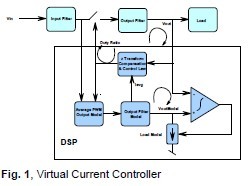
　　The portion labelled DSP represents difference equations solved within the DSP. An auxiliary control loop forces the estimated output voltage to be equal to the measured voltage by adjusting the load current. Then the average inductor curren tcurrent is made available to the duty ratio control loop. If the output filter uses measured output voltage, then a considerable simplification can be made as shown in Figure 2.

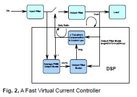
　　The duty ratio control loop is a modified PID controller where the differential signal is replaced by the average current. Separating the controller into an inner current loop and an outer voltage loop reduces the second order L-C filter to a first order system. It is useful to divide the code into separate plant and MPID models in order to handle the non-linear term resulting from multiplying the input voltage by the duty ratio. These 2 linear loops are then connected using the measured  input and output voltages and the previously calculated duty ratio. It can be seen that the MPID voltage loop is comparable to a PID control loop so that the extra complexity is all in the plant model.

　　1.1 Virtual Current Simulation Model

　　Figure 3 shows how the inductor current is solved. The Average voltage across the inductor is multiplied by the admittance of the filter inductor. Schematic parameters are used to calculate the various constants. The numerical values are　　inserted into the DSP code, using the schematic to replace the code header. Node vin1 is the A/D converter measurement of the output voltage and vxin is the product of input voltage and duty ratio; it is calculated based on the previous solution for duty ratio as measured using pwm1.

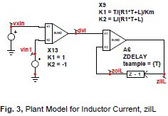
　　ZDELAY models the unit delay, eliminating solutions in between samples.

　　Next, the controller is modelled, borrowing the MPID topology. The PID constants are modified in summer X3. cuirin is the ziLL solution from the plant model and zivind1 is the reference minus the measured output voltage. Node naming rules are used to guide the code generator. These rules are error checked by the code generator.

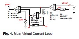
　　ZDELAY, A2, is an optional filter that is used if high ESR filter capacitors are used in the output filter. If the ESR is too large, the loop gain doesn’t fall off, causing high frequency instability. The X3:K3 term is used to make the inner current loop bandwidth about 1/3 the Nyquist frequency, damping the L-C resonance. The outer loop has most of the tolerance producing elements and its bandwidth is made to be about 7% of the Nyquiist frequency, yielding about 13 dB gain margin and 75 deg phase margin. Figure 5 shows a comparison of simulated and measured transfer function.

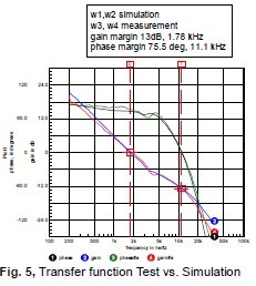
　　Both test and simulation use a single injection GFT approach described in [3]. The simulator runs an AC analysis and uses a script to plot and calculate the margins. The DSP measurement operates in time domain using a sine and cosine generating algorithm for loop excitation and average real-imaginary measurement [4]. Measurement are made for each of about 50 frequencies and returned to the IntuScope waveform viewer where the gain and phase is extracted and placed into vectors that are plotted upon completion of the frequency sweep. The hardware measurement takes about 20 seconds and the simulation runs in about 60 milliseconds, with an extra second for the used to press ‘b’ in IntuScope and view the bode plot results. This is the beginning of a new era when simulation performs hardware like functions faster than real time. Next, the transient response simulation and test results are compared in Figure6

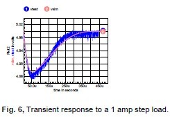
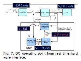
　　The measured data used an oscilloscope and shows the switching noise, which is averaged out in the simulation. An average transient can also be obtained from the hardware. Both AC and TRAN results agree within component tolerance limits. Figure 7 shows the steady state test point voltages obtained using the streaming test point option.

　　1.2 PID Simulation Model

　　The proportional integral differential, PID, model is widely used for digital control. It’s very simple and therefore has very fast execution time. For second order systems, it’s a pole-zero cancelling algorithm. Figure 8 shows its simulation model

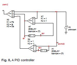
　　The pole-zero cancellation is imperfect because the digital control system zeros can’t match the analog R-L-C transfer function. Besides, the input filter characteristic makes the system greater than 2nd order. While PID gives good response to changes in setpoint, it exhibits ringing in response to step loads and is more sensitive to input fluctuations than current mode control. Figure 9 shows the bode plot and figure 10 is the transient response. The modification to make it an　　MPID controller consists of limiting the input error signal. That has the affect of limiting current and output overshoot at turn on. This limiting combined with proper integrator initialization eliminates the need for special soft start algorithms.

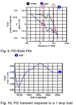
　　Both figures are scaled the same as figures 5 and 6 respectively. The pole-zero mismatch is evident in the Bode plot, while the load transient show the tendany to ring.

　　2. DSP Architecture

　　In general, both Texas Instruments and Microchip architectures have optimized the use of their respective processes to achieve a low cost, low power solution for SMPS applications. Clearly, it’s possible to make a Silicon solution that runs much faster, even using 64 bit floating point to avoid scaling issues. But that approach scales up cost and power leaving the low cost/power target market behind. Cost and power are minimized as word length and processor speed are reduced.　　That places a premium on design ingenuity to compete in this market place. Most contemporary low cost power electronics are produced using single sided PC boards. SMT technology is just emerging for these applications. Yes, that’s way behind the technology we’d like to use, however, price competition is a major consideration. DSP based designs are on the threshold of breaking into the low cost SMPS market. Both Microchip and Texas Instruments have a number of modules that perform a variety of peripheral operations like serial I/O; A/D conversion, pulse width modulation… Over time, nearly anything that used to be an external part has been drawn into the DSP so that very few peripheral parts need to be added. The PWM outputs still need drivers to interface with the power MOSFETS and there’s the need for interface buffers for communication with the outside world.

　　2.1. Texas Instruments Piccolo DSP

　　The Piccolo DSP has more RAM than Microchip. It takes advantage of the added RAM to run its program code from RAM for faster execution. TI uses a pipelined architecture, requiring a full pipeline to achieve throughput equal to its clock speed. The actual execution speed using a 60 mip chip is very close to the Microchip 40 mip chip.

　　The Piccolo A/D converter is 12 bits wide and advertised as an effective accuracy of about 10.6 bits. We measured 9.2 bits in our application, which could be because of PWM switch transinets. Noise appears to be normally distributed so that accuracy is improved by averaging many samples, thus increasing accuracy by the square root of the number of samples.

　　2.2. Microchip dsPIC33 DSP

　　Microchip has divided the RAM into XRAM and YRAM for the purpose of implementing the MAC instruction. This sits on top of an MPU architecture borrowed from the original Intel 80xxx series.

　　The XRAM, YRAM approach tends to make all memory look like registers; however, they still retain a preferred set of registers used for indirect addressing and multiplier, multiplicand storage. Microchip’s A/D converter is 10 bits wide we measured an effective 9.2 bits that performs adequately for PWM control, achieving 12 bit accuracy when averaged over 256 samples

　　2.3. Instruction set

　　1 Addressing

　　Both Microchip and TI have complex addressing modes that reduce the instruction count for common DSP operations. This is in contrast to the ARM7/9 architecture, also widely used in DSP’s that may require up to 3 instructions per clock cycle to achieve the same result.

　　2 The MAC Instruction

　　Both TI and Microchip have special hardware to implement the multiply accumulate, MAC operation. This added hardware is an important DSP feature that reduces the execution time needed to solve difference equations by a factor of about 3 over optimized C compiler execution. The implementation is slightly different, favoring Microchip for fewer clock cycles. The C-compilers for both products fail to use the MAC instruction for the following code, requiring assembly language coding to get the speed benefit. Microchip cannot shift right more than 8 bits; so a left shift (16-radix) is used instead by using the “sac” instruction that saves the upper accumulator word in a 16 bit register. The Microchip MAC, CLR and MOVSAC instructions are complex. After performing the operation, the multiplier and multiplicand registers are loaded from the pointer registers and then the pointer registers can be incremented or decremented by 2, 4, 6. Microchip addressing is byte oriented so that +=2 is equivalent to +=1 for C language or TI Assembly language. After performing a MAC product, the Microchip pointer registers are several memory locations ahead and the multiplier and multiplicand registers are holding data from the previous pointers. This makes assembly coding for Microchip very error prone. The TI MAC operation sums the previous product, requiring an extra summation at the end. Moreover, the TI shift operation requires loading the T register so that it really requires 2 instructions. The examples below are representative of what’s done by the Intusoft code generators. Further optimization may be possible by reusing the TI T and DP registers, combining pointer arithmetic for long sequences of null coefficients and taking advantage of the Microchip increment-decrement range. These added optimizations produce only modest speed improvements for the code examples provided with design-automated software.

C Language
Accum = 0;
Accum += *pState++ * *pCoef++;

Accum += *pState * *pCoef;
Accum = Accum >> radix;
Texas Instruments Assembly (n+4 + [1])
ZAPA
MAC P, *+XAR4[i],XAR7++
…
MAC P, *+XAR4[j],XAR7
ADDL ACC, P
MOV T, #8
ASRL ACC, T
Microchip Assy (n+2+[1])
clr A, [w8]+=2, w5, [w10]+=2, w6
mac w5*w6, A, [w8]+=2, w5,
[w10]+=2, w6
…
mac w5*w6, A, [w8], w5, [w10],w6
sac a, #-6 , w0
[1] Added instructions needed to reach nonsequential state locations
Moving Data
Both DSP’s have mov instructions. TI’s syntax is
<mov destination, source> ,
while Microchip is
<mov source,destination>.
TI can’t reach all memory with the mov instruction.So it becomes necessary on occasion to load the DP (Data Page) register in order to get the data ram in the proper page. The <@> symbol identifies the addressing method as DP relative. This is not very serious since most DSP instructions rely on registers and pointers that do access the entire RAM C Language
Accum = DSP_RAM_VALUE;
Texas Instruments
MOVW DP, DSP_REGISTER_BASE
MOV AL, @VALUE_OFFSET
Microchip
MOV DSP_REGISTER_VALUE, w0
Limiting Data
Keeping data within established limits is required to prevent arithmetic overflows. TI has MIN and MAX instructions that aid in limiting. However,each limit for TI takes 2 instructions while Microchip requires 3 instructions. HI and LO limits are usually required for each state variable, making the limit operations as costly as the MAC operations.

　　C Language

Accum > Hi ? Accum = Hi : Accum;
Accum < Lo ? Accum = Lo : Accum;
Texas Instruments
MOV AH, #HI ; biggest input in AH
MIN AL, AH ; if AL > AH, AL=AH
MOV AH, #LO ; smallest input in AH
MAX AL, AH ; if AL < AH, AL=AH
Microchip
mov #HI,w2 ; biggest input in w2
cpsgt w2, w0
; skip if biggest < measured
mov w2, w0 ; set lim val
mov #LO,w2 ; smallest in in w2
cpslt w2, w0
; skip if smallest > measured
mov w2, w0 ; set lim val

　　3. Comparative Test Results

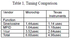
　　Each DSP was connected to the Intusoft Solar1TiM evaluation board. The 2 vendor DSP evaluation boards plug directly into connectors provided on the Intusoft evaluation board. Software for initialization and memory control was written in the C programming language. Interrupt service routines for the sine-cosine generator, the MPID control law and the Plant model were done in assembly language. In general, the C compilers worked well when the MAC capabilities were not required. Math operations were scaled using a mixed integer/fractional word. The binary point location was optimized for the problem at hand. For example, the sine-cosine generator used a 1.14 representation, where the number to the right is the number of binary bits in the fractional part and the left side accounts for the integer bits excluding the sign bit. The MPID algorithm used 7.8 scaling. The 10 bit Microchip A/D converter was scaled as though it was a 12 bit converter. MPID stands for Modified PID (Proportional Integral, Differential). Modifications are for limiting that provides automatic soft-start behavior. The control algorithms for the sine-cosine generator was hand crafted. Both the MPID and Plant models used DSP Designer Assembly language code generators

　　The Sine-cosine generator is used to generate the excitation signal for transfer function analysis and for the in-phase and quadrature signals used for signal detection.

　　An advanced virtual current controller used the plant model to estimate inductor current using a digital admittance model to estimate the inductor current. The MPID “differential” signal is replace by the estimated inductor current. The estimated current is also used to provide over current protection ; thereby eliminating the need for current sense components.

　　Timing was measured using an oscilloscope to measure the length of marker signals that were output at the beginning and end of each task.

　　4. Conclusion

　　The MPID control law runs about twice as fast as the virtual current controller. But the time required must include overhead for built-in test and background calculations. Overall the MPID controller runs about 30% faster than the virtual current controller. The additional speed translates into higher control bandwidth and smaller error from load switching. However, virtual current control eliminates the need for current sense components and can produce a critically damped response to output loads. The TI DSP is slightly faster but exhibits more virtual current noise when using its lower resolution pulse width modulator. Converting to the TI high resolution PWM should mitigate the noise problem albeit　　with reduced speed. Sample time for this test case was 15usec and the PWM period was 5usec. An analog solution runs at an effective sample rate of 200kHz or 3 times faster than the digital solution. Again that translates into smaller errors caused by load transients. Looking forward, Moore’s law works in favour of the digital approach, improving price-performance by a factor of 2 every 18 months. In a short time, the digital solution will be superior in terms of speed,　　parts count and cost. Plus, a digital solution adds a “smart” controller aspect that can adapt its behaviour to environmental changes and even recover from part degradation and heal some failures.

　　5. Literature

　　[1] Lawrence Meares: SPICE Simulation Provides Significan Advantages For a DSP Based SMPS: Power Electronics Technology Magazine: Part1&2: March-April 2009

　　[2] Lawrence Meares: AUTOMATING DIGITAL SIGNAL PROCESSING, DSP, DESIGN USING AUGMENTED SPICE SIMULATION, PCIM Europe 2009

　　[3] Intusoft Literature, GFTSummary.pdf, February 2003.

　　[4] Intusoft Newsletter: DSP Design Automation March 2010, NL83

　　[5] Microchip: dsPIC DSC High-Performance 16-Bit Digital Signal Controllers, 70155c.pdf

　　[6] Texas Instruments: TMS320C28x CPU and Instruction Set Reference Guide, spru430e.pdf 195